Tutorial:
Recommender Systems
May 20, 2022
Why Recommender Systems?

More Definitions
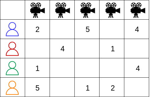
Explicit Feedback (or rating): Explicit rating given by the user for a product (e.g. star rating, thumbs up/down)

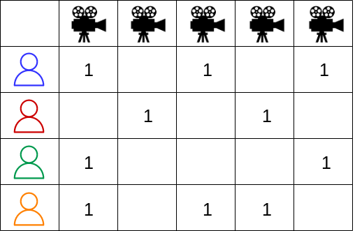
Implicit Feedback: Actions taken by the user which can be used infer preferences about products (e.g. click data, dwell time, purchases)
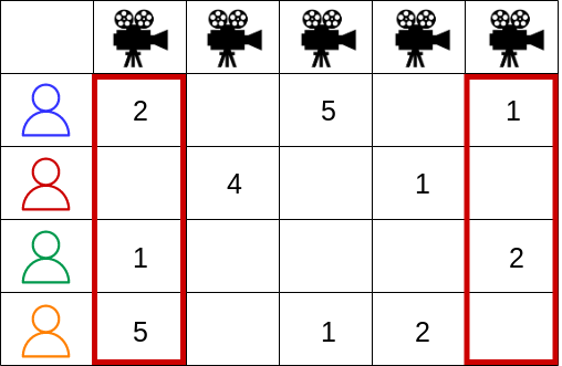
User-item Rating Matrix
User-item Rating Matrix (Implicit)
User-Item Matrix as a Bipartite Graph
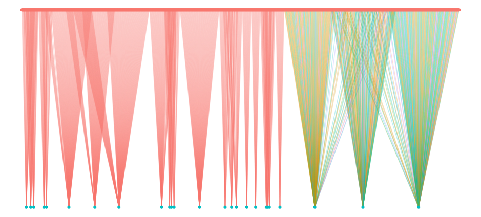
Items represented as blue nodes (bottom). Users represented as pink nodes (top). User-item interactions represented by an edge. Edges colored according to a particular user feature.
Recommender Technology Timeline
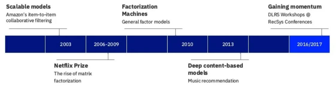
Presentation by Nick Pentreath at the 2018 Spark + AI Summit
2017 - 2022: Advances in deep learning for recommender systems.
![]()
Item-item similarity: Can be computed using cosine or Jaccard similarity, for example.
![]()
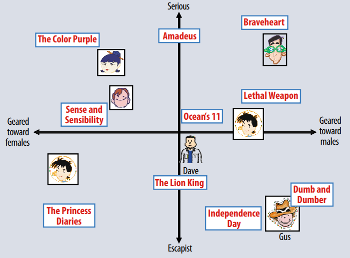
“Matrix Factorization”, a.k.a. latent factor model
Goal: Find user latent factor vector, \(p_i \in R^f\), and item latent factor vector, \(q_j \in R^f\), for each user and item. User’s rating of the \(j^{th}\) item: \(\hat{r}_{ij} = q_j^T p_i\)
Possible Solution: Compute the SVD of the user-item “matrix”.
Issue: How to impute missing values?
![]()
Goal: Find user latent factor vector, \(p_i \in \mathbb{R}^f\), and item latent factor vector, \(q_j \in \mathbb{R}^f\), for each user and item. User’s rating of the \(j^{th}\) item: \(\hat{r}_{ij} = q_j^T p_i\)
Better Solution: Model ratings and solve via stochastic gradient decent or alternating least squares.
\[ min_{\substack{p,q}} \sum_{(i,j) \in \kappa} (r_{ij} - q_j^T p_i)^2 + \lambda (|| q_j ||^2 + || p_i ||^2) \]
![]()
\[ min_{\substack{p,q}} \sum_{(i,j) \in \kappa} (r_{ij} - q_j^T p_i)^2 + \lambda (|| q_j ||^2 + || p_i ||^2) \]
Enhancements:
- Incorporate global and main (user, item) effects
- Incorporate confidence weights for implicit feedback
- Model as a function of time
- Ensemble many models
![]()
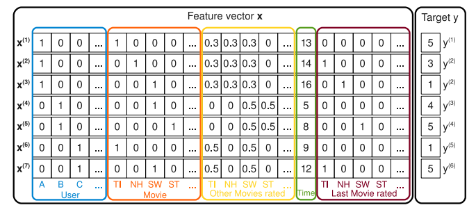
Hybrid model inspired by support vector machines (SVM) and matrix factorization.
\[ \hat{r}_{ij} = w_o + \sum_{i=1}^n w_i x_i + \sum_{i=1}^n \sum_{j=i+1}^n x_i x_j {\bf v}_i \cdot {\bf v}_j \]
![]()
Example: Pandora uses content associated with music that the listener has liked to recommend new music.
- Old: “Musicologists” manually entered features about songs (mood, tempo, artist, etc.)
- New: Deep content models learn features from music audio
![]()
- 2016-2017: Deep Learning for Recommender Systems (DLRS) Workshop at RecSys Conferences
By 2018 the DLRS workshop was discontinued in favor of presenting deep learning work in the main part of the conference.
Today: State-of-the art deep learning for all types of recommender systems.
Matrix Factorization in a Deep Learning Framework
Loss function: MSE
NCF
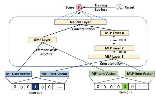
- Previous RecSys Model for MLPerf
- Collaborative filtering only (no side features)
Wide and Deep

- Model from Google
- Memorization + Generalization
- Example: App recommendation. Input: Item indices, user side & context info. Output: Binary (indicating app installation)
DeepFM
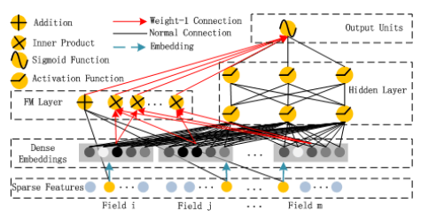
- Model from Huawei
- Inspired by Factorization Machines
- Example: Criteo dataset (13 integer-valued features, 26 categorical features, binary labels)
DLRM
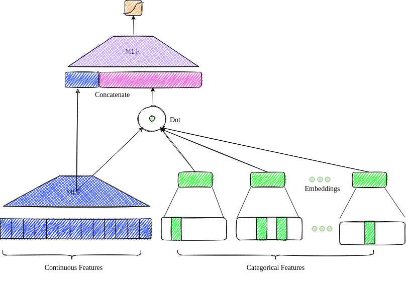
- Model from Facebook
- Current MLPerf RecSys model
DCN-V2
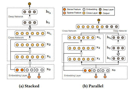
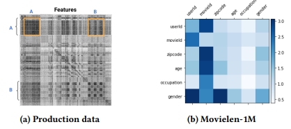
DCN-V2: Under the Hood
We can consider the weight matrix W in the first cross layer.
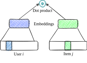
Terminology: Two-tower Systems

Used for item retrieval (as opposed to ranking).
Challenges of News Recommendation
- Severe cold start problem: New articles posted continuously. Usefulness of articles diminishes quickly.
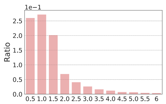
- Survival time of more than 84.5% news articles is less than two days.
- Estimated using the time interval between first and last appearance time of articles in the MIND dataset.
NRMS
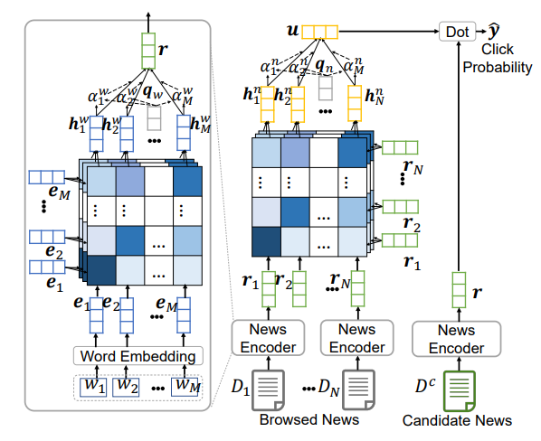
- Model from Microsoft
- Best performing model in the MIND paper.
Evaluation Metrics for Recommendation Systems

- Hit Rate at \(k\) (HR@\(k\))
- Mean Average Precision at \(k\) (MAP@\(k\))
- Normalized Discounted Cumulative Gain (NDCG@\(k\))
- Mean Reciprocal Rank (MRR)
- Diversity at k (Div@k)
- Novelty at k (Nov@k)
- Catalog coverage (CC)
Unlike accuracy metrics, which are computed using a test set, beyond-accuracy metrics are computed on the final recommendation list.
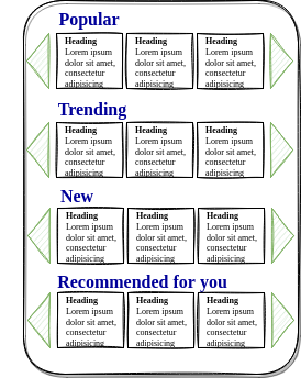
More Tips
Personalized recommendations in conjunction with other types of recommendations can provide a satisfying user experience.
![]()